Data Exploration

Locating Data

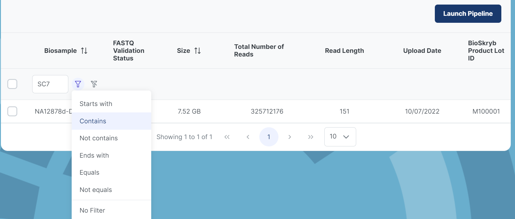
Within each project, you can search for biospecimens at the header row. There are 2 icons next to the search box that look like funnels. The one on the left will filter your search based on the following parameters shown in the 2nd picture below. The funnel on right that has a slash through it will not filter your search and will look for a Biosample based on the exact name.

Pipeline Outputs

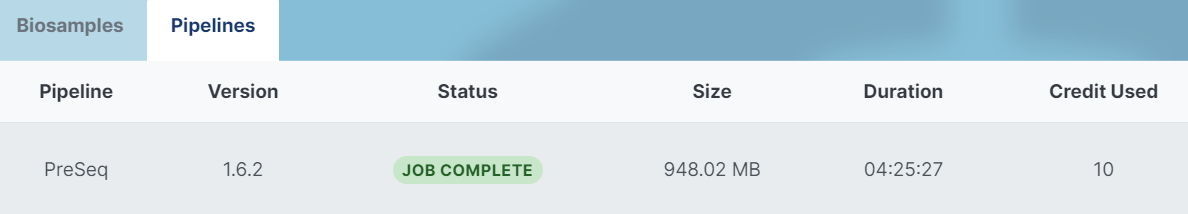
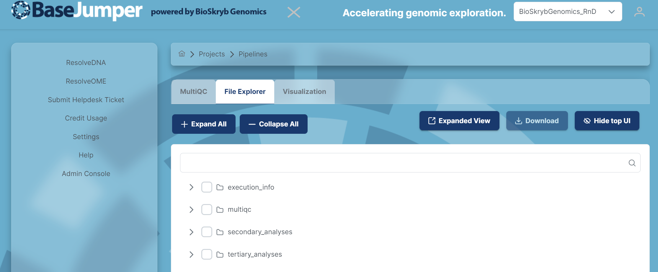
When in pipeline view, click on the previous pipeline launched and a page will pop up with 3 different options: MultiQC, File Explorer and Visualization. You can select the tab for file explorer and search for biosample, ID or file extension to bring one or more files visible in the file explorer. The file explorer contains multiple sub folders for several output files. To find the specific files needed for your experiments, see the Pipeline Docs section and go to your specific pipeline. The output files section of these documents will summarize the main output files contained in each sub folder in the file explorer. More instructions on this can be found in the Data Export section.

Data Visualization

In BaseJumper we have built in downstream analysis software to make it easier for you to analyze your data. We have embedded the Integrative Genomic Viewer(IGV), Copy Number Variants(CNV), Variant Filtering and other visualization apps. This is designed for all pipelines in BaseJumper. In this section we will go over how to use the visualization tools in BaseJumper.

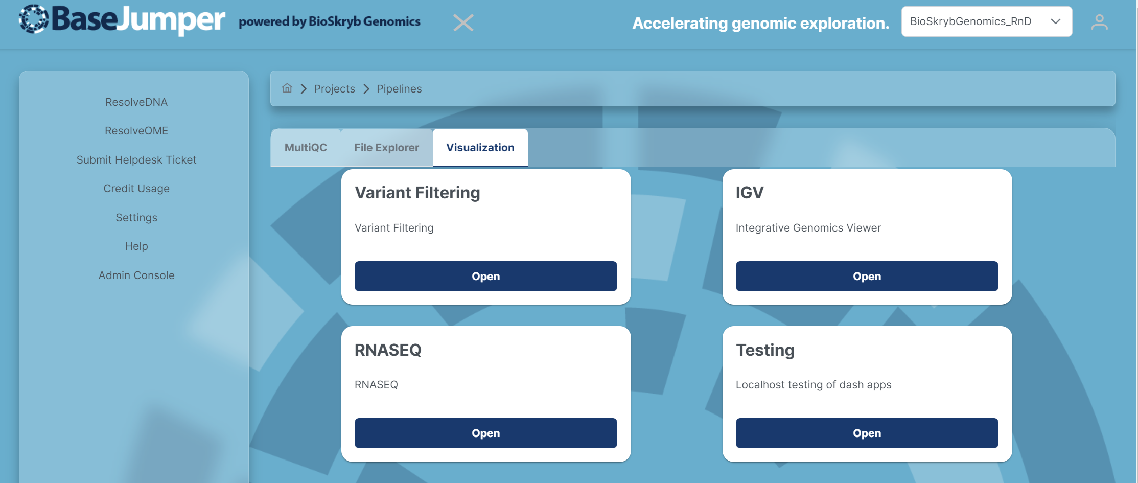
To access the visualization tools, click on the Visualization tab and a few different options for visualizations will appear for you to choose from.

IGV App

1. IGV is a visualization tool used to analyze Genomic datasets and identify different types of variants and mutations cross the genome whether that is a insertion, deletions, etc. For more information on how to use IGV go here.

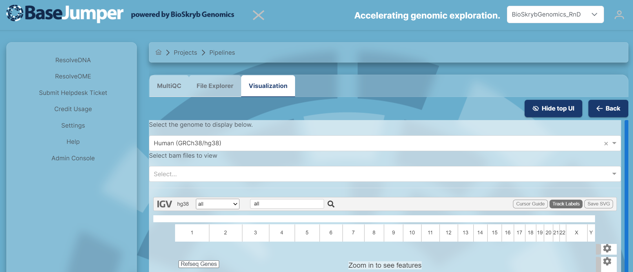
   To access the Integrative Genomic View, click on the Open button in the IGV tab and the IGV software will appear.

2. First select the Genome that you want to use for the visualization. The default will be Human(GRCh38/hg38).

   

3. To view samples in IGV, you have to input bam files. Each sample in this visualization will be in the .bam format. In the 2nd pull down bar, where it says Select bam files to view select the Biosamples that you would like to look at for your analysis.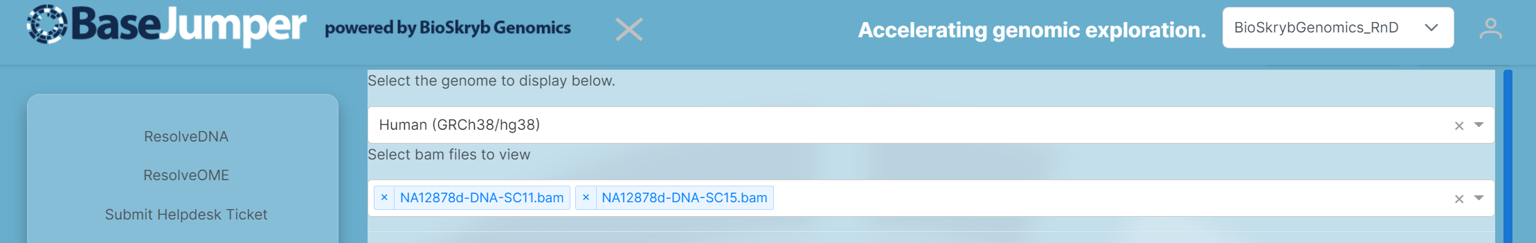

   

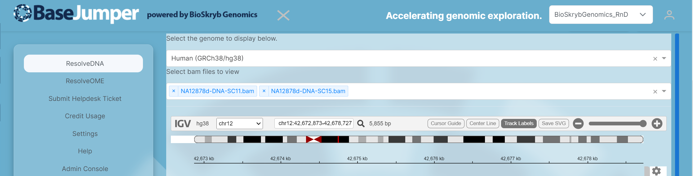
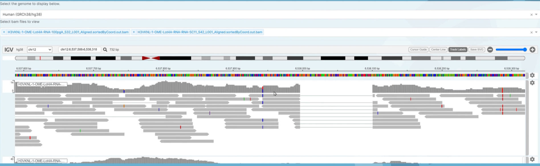
4. Next, select the chromosome that you want to specifically look at. Then, you can zoom in and out to look at the reads for each sample by maneuvering the zoom tool (has a plus and minus sign) or you can search for your gene of interest in the search bar next to the magnify glass. There are also options to add track labels(name of each individual sample), center lines and a cursor guide. These options are on the right of the IGV tool bar next to the zoom tool.

   

5. You will then see the reads appear and you can start comparing and contrasting the different mutations found in the different samples across the genome.

6. If you want to save these these images to your computer, click on the save SVG button next to the zoom tool. This will be saved as an .svg file and will download directly to your computer.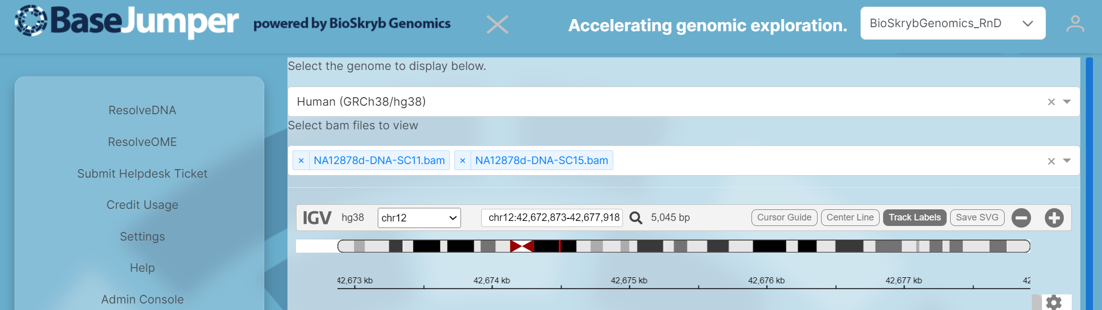

   

CNV App

This Copy Number Variants tool is now embedded in Base Jumper platform.

1. To access the CNV tool, click on the Open Button under the CNV tab.

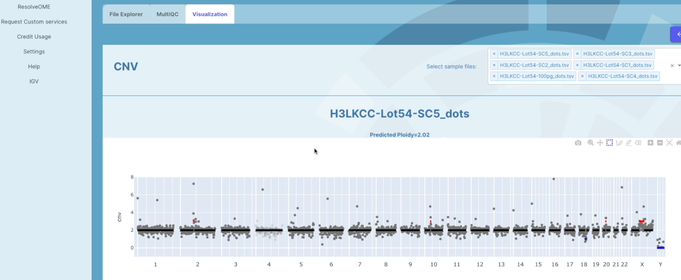
2. A CNV graph will appear and in the upper right hand corner a list of all sample fields will be displayed. If you need to remove or add a sample, you can click on the X to remove a sample or the down arrow to add a sample. A drop down box will appear and you can select the samples that you want to view.

3. The CNV graph is made for each individual sample. The overall ploidy across the genome will be shown at the top of the graph for each individual sample. The individual grey dots represent physical regions within each chromosome. The X axis shows the 22 autosomes and the 2 sexual chromosomes. The Y axis shows the estimated ploidy level across each chromosome. The change in different regions are shown in the solid black line. The red dots represent gains and the blue dots represent losses. These variants are shown through out every chromosome.

   

4. If you want to look at specific regions within a cell, click on the square box in the upper right tool bar on the graph. You can then use the square tool to select the region that you want to look deeper into.

   

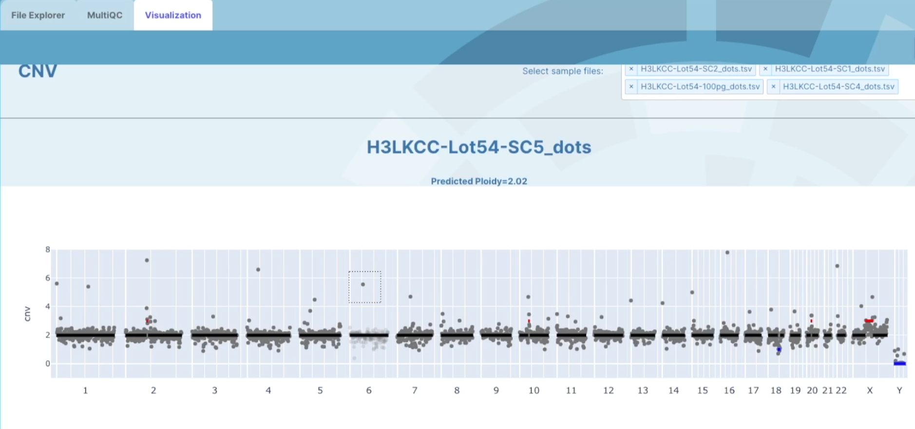
5. At the bottom of the graph, you will see displayed a table with a list of genes across your selected region that shows were each gene's location starts and finishes, the gene-id, and the ploidy number. This table also has filter options for you to filter genes by gene of interest. There is also an option to download a list of the genes from that region by clicking on the download genes button and this will download to your computer as .txt file.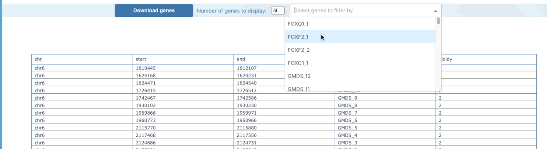

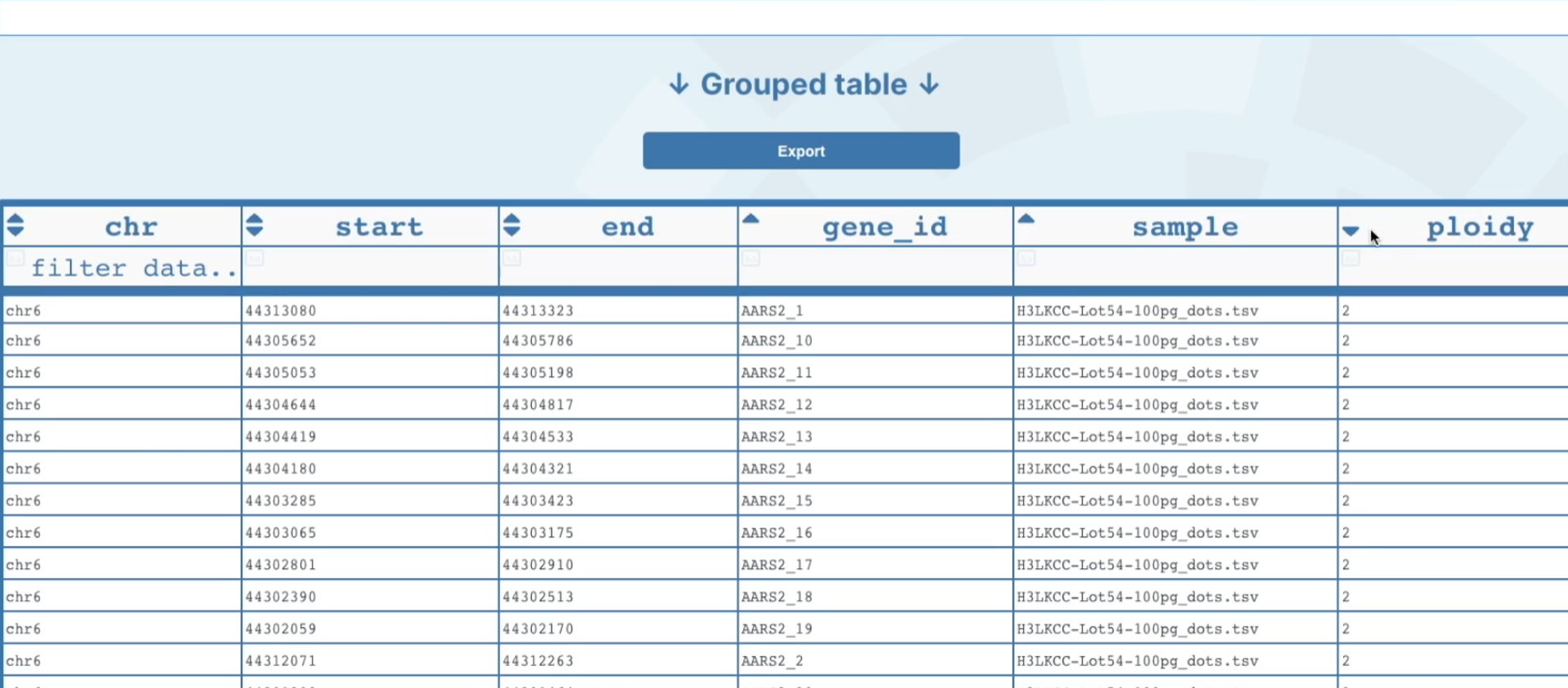
6. At the bottom of the page there is an option to view all genes across the whole genome in the Grouped table. Each column has an option to filter based on certain parameters in order to find your gene of interest. This group table can also be downloaded by clicking on the export button at the top of the table and a .tsv file will be downloaded to your computer.